Gradient Descent
What does Gradient Descent do
It minimizes cost function using derivatives by proceeding in epochs (an epoch consists of using the training set entirely to update each parameter).
Adaptive methods
The adaptive methods in gradient descent can automatically adjust the learning rate.
- Newton's method
- computes and uses the full Hessian
- works for convex problems but needs adjustments for nonconvex problems
- preconditioning
- avoids computing the Hessian in its entirety but only computes the diagonal entries
Gradient Descent in Neural Networks
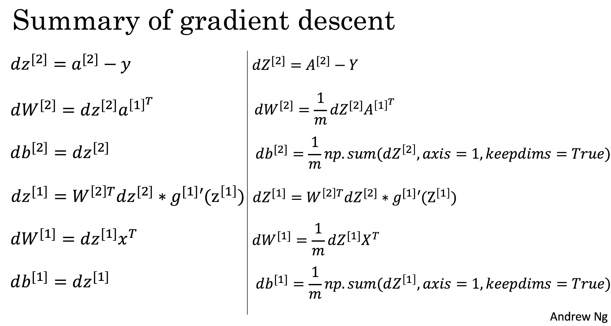
Gradient computation
- use forward-propagation to calculate the values of each layer
- use back-propagation to calculate the derivatives
- example of a two-layer logistic regression neural network (by Andrew Ng):
Challenges and Solutions
Vanishing / Exploding gradients
Challenges
- Vanishing gradients
- the gradients of a neural network's loss function become extremely small
- causes the weights to update very slowly and making it difficult for the network to learn effectively
- Exploding gradients
- gradients become excessively large
- leads to unstable updates and causing the model's parameters to oscillate or diverge during training
Solutions: Initialization (Starting Point for Gradient Descent)
- Initialization = refers to how the network’s weights are set before training begins.
- Common initialization strategies:
- Xavier/Glorot Initialization: tailored for tanh activations; for balanced signal flow
- He Initialization: tailored for ReLU activations.
- Pretrained weights: from transfer learning or self-supervised learning.
- bias terms are often initialized to zero or small constants.
Optimization is too slow
Challenges
- Model convergence can be slow or stall due to:
- Poor gradient flow
- Suboptimal hyperparameters
- Lack of normalization or regularization
Solutions
- Gradient checking
- use only for debugging gradients (e.g., to verify backpropagation implementation)
- ensure to include regularization terms in the check
- doesn't work for dropout
- Hyperparameter Tuning: Hyperparameter Tuning#Hyperparameter Tuning in Deep Learning
- Batch Normalization: Regularization#batch-normalization
Variants of Gradient Descent
Variants Outline:
-
[[#Batch gradient descent]]
-
[[#Stochastic gradient descent (SGD)]]
-
[[#Mini-batch gradient Descent]]
-
[[#Momentum]]
-
[[#RMSprop (Root Mean Square prop)]]
-
[[#Adam (Adaptive Moment Estimation)]]
-
[[#Learning rate decay]]
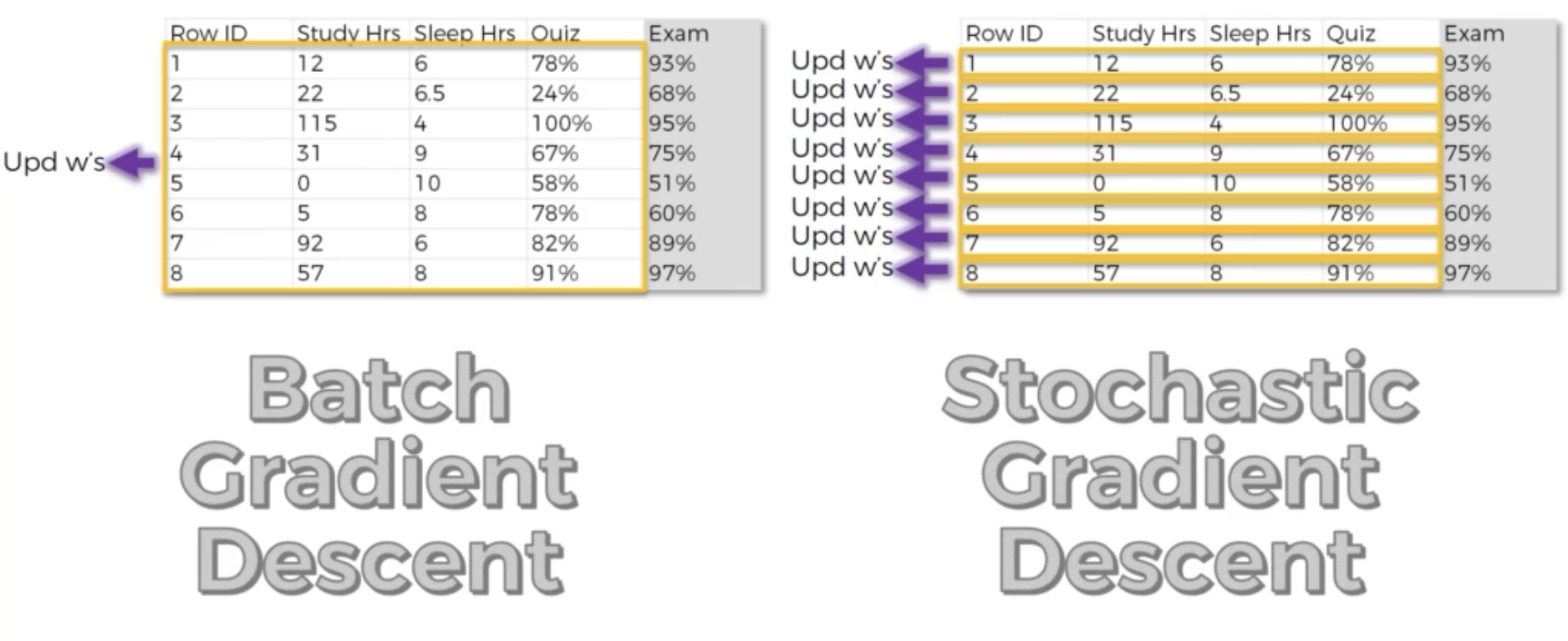
Batch gradient descent
- most basic approach
- the loss function= an average of the losses computed on every single example in the dataset
Stochastic gradient descent (SGD)
- a variant of batch gradient descent where the weights are updated after computing the gradient of the loss function with respect to a single training example at a time
- while each individual observation will provide a poor estimate of the true gradient, given enough randomness the parameters will converge to a good global estimate
- SGD itself has various “upgrades” variants
- AdaGrad
- a version of SGD that scales
for each parameter according to the history of gradients. As a result, is reduced for very large gradients and vice-versa - used per-coordinate scaling to allow for a computationally efficient preconditioner
- a version of SGD that scales
- Momentum (Gradient Descent#Momentum): helps accelerate SGD by orienting the gradient descent in the relevant direction and reducing oscillations
- RMSprop (Gradient Descent#RMSprop (Root Mean Square prop)) and Adam (Gradient Descent#Adam (Adaptive Moment Estimation)): frequently used in neural networks
- AdaGrad
Batch gradient descent vs. Stochastic gradient descent
- batch ones are slow; stochastic ones can avoid local minimum but can be noisy and computationally inefficient
- different ways to update weights
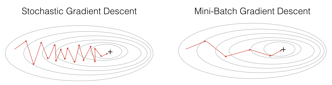
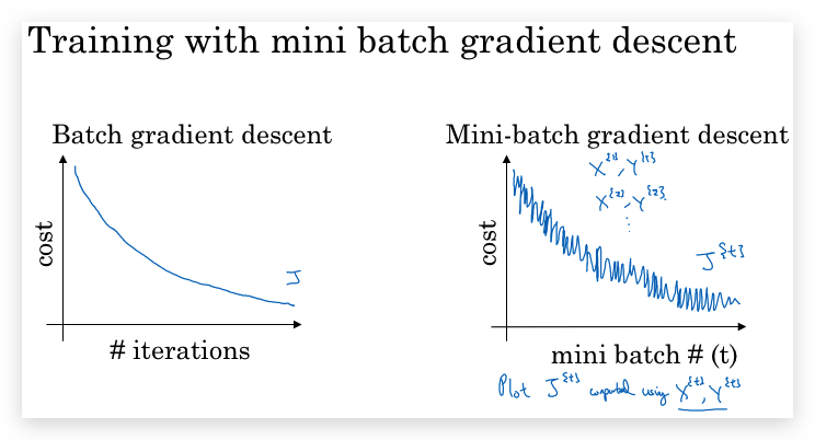
Mini-batch gradient descent
- Mini-batch a compromise between batch and stochastic gradient descent, where the weights are updated after computing the gradient of the loss function with respect to a small batch of training examples (typically between 32 and 512).
- efficient multi-machine, multi-GPU and overall parallel processing
- Comparison: SGD vs. mini-batch gradient descent
- when to use
- when the data size is very large (>= 2000)
- what to use
- if
= m: batch gradient descent - if
= 1: stochastic gradient descent - usually
: 64, 128, ...
- if
- it should fit in CPU/GPU memory
Exponentially weighted averages
(Exponentially weighted moving averages)
- describes the trend using local averages
Momentum
- The idea behind gradient descent with momentum is to add a "momentum" term to the weight update rule (stochastic gradient descent) that encourages the weight updates to continue in the same direction as the previous updates
- it aggregates a history of past gradients to accelerate convergence and reduce oscillations in the optimization process
- The weight update rule for gradient descent with momentum can be written as:
where
- v(t) is the "velocity" vector at time t
is the momentum coefficient (typically set to a value between 0.9 and 0.99) - learning rate is the step size or learning rate
- gradient is the gradient of the loss function with respect to the weights
- weight(t) is the weight vector at time t
RMSprop (Root Mean Square Prop)
- it works by maintaining a moving average of the squared gradients and using that to scale the learning rate
- it decouples per-coordinate scaling from a learning rate adjustment
- coefficient
determines how long the history is when adjusting the per-coordinate scale
Adam (Adaptive Moment Estimation)
- Adam is a combination of two other optimization algorithms, namely, stochastic gradient descent with momentum and RMSprop.
Learning rate decay
- reduce the learning rate over time as the optimization process progresses.
- the idea behind learning rate decay is that as the algorithm gets closer to the minimum of the loss function, it may benefit from smaller steps to avoid overshooting or oscillations around the minimum.
- can be combined with other algorithms such as SGD and Adam